Assessment of the Value of New Information to Inform Water Quality Management Decisions

It is typical for decisions on the management of surface water quality to impact several environmental, social, and economic factors or attributes important to the public. In theory, this can lead to a difficult and complex problem analysis, but in practice many factors are virtually ignored during analysis and decision making. Further, it is typical for the predictions of the impact of proposed management actions on these attributes to be highly uncertain. Often it is possible to reduce that uncertainty through additional research and analysis, but resources for this are scarce and decision makers may not be inclined to wait for these results as they seek action and quick problem solution.

In part to provide the scientific basis for problem solution and action, a variety of simulation models have been developed, yet increasingly it is being recognized that these models are not very reliable. As a consequence, whether it is the initial intent or not, successful management often involves judgment-based decision, followed by implementation, feedback, and readjustment. This “learning by doing” approach is a pragmatic attempt to deal with growth, change, new information, and imprecise forecasting.

Learning by doing, or adaptive management, is a strategy that treats management as a continually ongoing process utilizing observation and feedback. Management actions may change, or adapt, to the observational feedback; rather than create an elaborate model a priori and base all subsequent decisions on predictions from that model, the adaptive approach emphasizes updating of a model based on observation and learning as time passes. Updating the model may be done informally or formally through the use of statistical methods, and management actions can then be adapted to be consistent with the predictions of the revised model.

This adaptive approach may be particularly appealing in situations where population growth, land use change, and variability in climatic forcing functions exceed the limited realm of current observation and experience. Such systems involve complex and often highly nonlinear relationships among various elements; prediction in these chaotic environments can be difficult in the short term and useless in the long term. Even state-of-the art models of such systems require periodic observation, evaluation, and revision in order to improve predictive validity.

Consider the USEPA TMDL program, where the often-substantial uncertainties in water quality forecasting, the practical difficulties in comprehensive error estimation and propagation, and the inadequate approaches for TMDL margin of safety estimation are each compelling reasons to consider a new approach to TMDL assessment and implementation. These problems are not merely of academic interest; rather, they are indicative of flawed TMDL forecasts, leading to flawed TMDL plans. The consequence is that TMDLs will often require re-adjustment.

These forecasting difficulties formed the basis for the 2001 NRC panel recommendation for adaptive implementation of TMDLs. Stated succinctly, if there is a good chance that the initial forecast will be wrong, then an appropriate strategy may be one that, right from the start, takes into account the forecast error and the need for post-implementation adjustment. Decision analysis provides a prescriptive framework for this type of assessment.

In a decision analytic framework, scientific research and monitoring studies in support of environmental management should be selected on the basis of an assessment of the value of information expected from completion of the study.  In general, scientific investigations should be supported if the value of the expected reduction in prediction uncertainty appears to justify the cost of the scientific analysis. In a formal decision analysis, one could estimate the change in expected utility associated with the cost of additional investigations, the deferral of decision making until new analyses are undertaken, and the reduction in prediction uncertainty.

An assessment of cost versus uncertainty reduction can be made in a formal, rigorous sense using decision analysis. If a simulation model is selected as the predictive framework for TMDL development, sensitivity analysis might be applied with the model to estimate the relative magnitude of uncertainties. Alternatively, if sensitivity analysis is not feasible, expert judgment may be used in conjunction with the model to define scientific uncertainties that appear to have the greatest impact on prediction error. If cost is acceptable, research and/or monitoring to improve scientific understanding may then be directed toward reducing those uncertainties and ultimately updating the model forecast.

Consider the following hypothetical example. New scientific information to reduce uncertainty in the prediction of chlorophyll a in Lake Okeechobee using WASP (Water Analysis Simulation Program) is being considered. In particular, we are interested in research and monitoring projects that can be completed within a designated time period and that contribute to the reduction of prediction uncertainty, leading to a revised model and an improved forecast. By “project” I mean any research or monitoring program, such as pollutant/criterion monitoring, evaluation of the effectiveness of a BMP, or a research experiment to improve a model parameter estimate, that can improve the post-implementation assessment of the response variable (chlorophyll a).

An expected utility framework is proposed to relate prediction uncertainty reduction (weighted by the probability of successful completion of the project), project cost, and other research evaluation criteria on a common valuation scale. The result is a priority list for proposed scientific research and monitoring activities that can support an analytic approach for adaptive implementation of a TMDL. While this example is presented within the framework of an adaptive TMDL, it is important to emphasize that it is quite general; indeed, the example below was actually conceived and proposed for the South Florida Water Management District outside of the TMDL program.

Water quality standards, which consist of a designated use and a criterion, provide the foundation for a TMDL. If measurement of the criterion indicates that a standard is violated, then a TMDL must be developed for the pollutant causing the violation. In most cases, a water quality model is used to estimate the allowable pollutant loading to achieve compliance with the standard.

The criterion of interest here, chlorophyll a concentration, may be affected by a number of management options; certainly one of the more likely options for limitation of algal concentration is to regulate land use for nutrient load controls. Now, in order to predict the effect of a land use control option on chlorophyll a, the scientist must link land use and chlorophyll in some way (perhaps through a mechanistic model, or through a statistical model, or through expert judgment). The analysis presented here is based on the assumption that this link for Lake Okeechobee eutrophication management will be the simulation model WASP.

Thus, WASP provides the comprehensive predictive framework (when linked to an assessment of the relation between land use and nutrient loading to the lake) for assessing the impact of management actions on the chlorophyll criterion. Any proposed scientific investigation (research and monitoring) designed to improve the prediction of the impact of management decisions should be selected using WASP as the evaluation framework. Also, research should not be guided toward scientifically interesting questions or motivated by the desire simply to improve scientific understanding, unless this additional scientific knowledge is justified in an evaluation using the WASP predictive framework.

For example, ecologists may be quite uncertain concerning the role of zooplankton grazing on phytoplankton density and chlorophyll a. Further, it may be believed that this phytoplankton loss term is extremely important in some lakes. Formal or informal analysis of research projects using the predictive framework (e.g., WASP) may then be used to determine:

• Can research successfully be completed within a specified time frame to reduce uncertainty concerning the effect of zooplankton grazing on chlorophyll in the lake?
• What is the expected reduction in prediction uncertainty, for the chlorophyll criterion, associated with a proposed zooplankton grazing research project?
• Is the uncertainty reduction versus cost ratio for this project favorable relative to other proposed research and monitoring projects?

The utility-based method proposed below may be used to conduct this analysis.

In summary, for this case study on Lake Okeechobee, an expected utility framework is proposed to assess the value of monitoring/research in improving predictions. Application of this approach is quite general; it could serve to prioritize studies for initial model development, or it could be used for iterative improvement of a model and its forecast, as in an adaptive TMDL.

If it is assumed that uncertainty reduction and project cost are judgmentally independent, then an additive utility model (see the equation below) may be a reasonable approximation for the valuation model. Judgmental independence may be assumed for two attributes if value judgments can be made about each attribute separately. For example, project cost and uncertainty reduction are usually related, since project options can often be identified for which uncertainty reduction increases with project cost. However, it is likely that judgments (not tradeoffs) concerning the relative value (or loss) due to project cost, and the relative value of uncertainty reduction, can be made separately. Thus, for a particular scientific research or monitoring project, aj, the expected utility (EU) of the project is estimated as:

where Ui(xi) is a utility measure (i.e., a scale reflecting value) for the ith attribute, which

might be uncertainty or cost; wi is a weight on  the ith attribute; and pi is the estimated probability that the proposed project will yield the expected level (x) for the ith attribute (e.g., what is the probability that the expected 20% uncertainty reduction will be achieved?). Note that the cost attribute may often have a probability of one (indicating that the estimated project cost is expected to be realized). The additive model in Equation 1 is a reasonable, but certainly not the only, approach to combine information and rank proposals.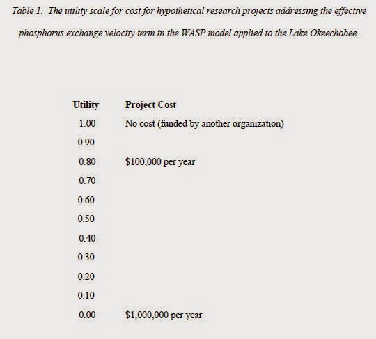

To use this equation, the attribute scale (e.g., dollars for project cost, percent error for prediction uncertainty,...) must first be translated to a 0-1 utility scale reflecting value. This scale provides a common metric for all attributes; examples are given in Tables 1 and 2. 


Weights are then assigned to each attribute reflecting relative importance and also reflecting the approximate range on the magnitude of each attribute. Relative importance is simply a measure of the significance of each attribute to the decision. Range is important because, if all projects have exactly the same cost (zero range), then cost is irrelevant as a decision making attribute. Once this general scheme is established, any particular research or monitoring project can be assessed in a straightforward manner.

Application of this project evaluation scheme requires involvement of both scientists and decision makers. The scientists' role is to: (1) propose research and monitoring projects, (2) evaluate project success (e.g., uncertainty reduction and probability) and cost, and (3) assess WASP prediction error reduction. The role of the decision makers is to: (1) determine project evaluation attributes (e.g., uncertainty and cost), (2) define the utility scale for each attribute, and (3) determine relative weights for the attributes. Interactions between scientists and decision makers is apt to be helpful for the tasks of each group; however, it is important that each group fulfill its responsibility. It makes little sense for a nonscientifically trained decision maker to design a ecological research project. Likewise, it makes little sense for a nonelected or nonappointed scientist, unfamiliar with public and decision maker values, to define the utility scales for prediction uncertainty reduction and for cost.

To begin the project assessment, the level (or magnitude) of each attribute must be estimated for the project of interest. For example, research/monitoring cost would be estimated in the usual way and then converted to the utility scale for cost. Prediction uncertainty, however, is likely to be more complicated. First, the uncertainty in the quantity of direct interest in the proposed research or monitoring project must be estimated. Thus, if research is designed to reduce the uncertainty in the WASP phytoplankton settling velocity parameter, the expected reduction in uncertainty in this parameter must be estimated. Once the parameter uncertainty is estimated, it must be converted into a reduction in prediction uncertainty for the attribute (e.g., chlorophyll) of interest. This conversion may be accomplished with sensitivity analysis using WASP or may be based on expert judgment by a scientist familiar with WASP and ecological processes in Lake Okeechobee. Next, the prediction error reduction estimate is converted to the utility scale. The utilities for all attributes are weighted, then multiplied by an estimated probability of achieving the expected attribute level. The final step is summation of the probability-weighted utilities.

While these uncertainty estimates and project success probabilities are useful measures of the value of research/monitoring, they are not routinely estimated in research/monitoring design. Nonetheless, these terms must be estimated to carry out the proposed project evaluation scheme. Scientists may be uncomfortable with this quantification requirement; however, they must recognize that their recommendation in support of a research or monitoring study to guide environmental decision making is tantamount to a favorable project rating using a scheme like that in Equation 1. Reduction in scientific uncertainty and probability of project success are implicit in any project recommendation.

Assume that the predicted in-lake sediment phosphorus flux rate based on the application of WASP to Lake Okeechobee is quite uncertain, and phosphorus release from the lake sediments is thought to be an important contribution to chlorophyll development. The expression in WASP for sediment phosphorus flux rate is (in g/m2-day):

where EDIF is the diffusive exchange coefficient (in m2/day), Dj is the benthic layer depth (in meters), DIP is dissolved inorganic phosphorus (in g/m3), DOP is dissolved organic phosphorus (in g/m3), j refers to the benthic layer, and i refers to the water column. The two uncertain parameters of interest, EDIF and Dj, are likely to be correlated, and it is likely that their combined effect can be more precisely estimated than can the combination of their separate effects. Thus, proposed research is designed to estimate the quotient of the parameters:

where vp is an effective phosphorus exchange velocity term (in m/day).

Based on current knowledge, the uncertainty in vp can be expressed in percent error, with one standard error estimated to be about ±40% (i.e., there is about a 2/3 chance that ±40% bounds the error). This error estimate reflects both scientific uncertainty and natural variability. Research is proposed involving in situ sediment phosphorus flux studies at randomly selected locations over a three-year period (in the hope of observation during a range of meteorological and hydrological conditions) at a cost of $150,000/year. Scientists expect these studies to reduce the error in vp by one-half (from ±40% to ±20%). However, the scientists acknowledge that they have a few concerns about research methods and possible problems in the field, so they have set the probability of research success (defined as achieving the expected reduction in uncertainty) at 0.8. The probability that the project will cost $150,000 as expected is set at 1.0.

While research is focused on improved estimation of vp, this research has management interest because it is expected to reduce WASP prediction error for the chlorophyll attribute. To estimate the prediction error reduction, Monte Carlo simulation can be used with WASP to determine the effect of a reduction in error in vp from ±40% to ±20%. Alternatively, expert judgment from a scientist familiar with WASP and with ecological processes can be substituted if WASP is not satisfactorily calibrated for the application. The latter option was chosen here, and the expert estimated that the expected reduction in vp error would reduce the WASP prediction error for the chlorophyll attribute by 5%-10%.

All necessary information has been obtained, so utilities can be estimated and Equation 1 can be applied. Based on Tables 1 and 2 (which are to represent the value judgments of decision makers), the utility for cost appears to be approximately 0.7, and the utility for prediction uncertainty reduction appears to be about 0.4. The decision maker in this case assesses the weight on the prediction uncertainty attribute to be about three times larger than the weight on cost; therefore, the uncertainty weight is 0.75 and the cost weight is 0.25. Applying the equation, the expected utility of the project (a1) is:

The utility for all other proposed projects addressing the chlorophyll attribute can be determined in the same way and then compared to yield a relative ranking on the expected utility scale. Research and monitoring projects with the highest expected utilities should have the highest priority for support.

The analysis that is presented here is hypothetical while still intended to describe how improvements to models might be rigorously assessed. Nonetheless, one must acknowledge that it is quite possible that any individual experiment or monitoring project will contribute only a relatively small amount to uncertainty reduction. Further, the value of information calculations described above may be quite uncertain in practice. For large process models the sensitivity analyses may be difficult, as correlations between model terms may be important yet difficult to estimate. Nonetheless, as already noted, the decision to conduct additional monitoring or research to improve the scientific basis for decisions carries with it, at a minimum, an implied acknowledgment that the benefits of new scientific information justify the costs.

In practice, a number of the choices and issues that make up this analysis are far from straightforward. For example, a proposed project can serve to improve the assessment of compliance with a water quality standard (i.e., learning) and/or can serve to actually achieve compliance (i.e., doing). Thus, some projects (e.g., an improvement in wastewater treatment efficiency) might be implemented solely as management actions and would be implemented with/without the adaptive management learning opportunity. Other projects (e.g., a monitoring program to assess standards compliance) are implemented solely to assess the effectiveness of management actions. Still other projects (e.g., implementation of a particular agricultural BMP) might serve both purposes. For the purposes of the value of information analysis proposed here, the relevant project cost is that which relates to the learning objective.

In estimating the value of research, experimentation, and monitoring, the decision maker must assess the utility for reduction in TMDL forecast uncertainty. Some decision makers may be able to directly consider the merits of uncertainty reduction, but many probably will not. For a decision maker, reduced TMDL forecast uncertainty is meaningful when translated into social and economic consequences, but these may not be readily apparent. Thus, for this proposed value-of-information scheme to work effectively, the analyst should be prepared to discuss the expected outcomes associated with reduced uncertainty to stimulate thinking on the part of the decision maker concerning the socioeconomic consequences of “good/bad” decisions. Similar difficulties are likely to be encountered when the decision maker estimates the weights on the attributes. Fortunately, there are ways to present the cost/uncertainty trade-offs that may result indirectly in the estimation of these weights. In sum, these are difficult choices, and many decision makers lack experience with these choices; however, that does not change the fact that implicit in decisions to undertake/forego new information gathering is an assessment of these terms in this decision model.

Finally, there may be essentially an unlimited number of projects that might be considered for learning; in practice, it is feasible to rigorously assess only a handful. It seems reasonable to assume that scientists and water quality modelers will be able to identify proposed management actions that have the greatest uncertainty concerning impacts, they should know the uncertainty in the forecasted outcome (and can easily compute the value of compliance monitoring), and they should know (or be able to assess) the weakest components of the model that might be improved with experimentation. Thus, in practice, we are likely to depend on the judgment of the scientific analysts to identify a relatively small number of options for consideration in this procedure.

The expected utility analysis described here can help prioritize proposed research and monitoring to reduce uncertainty in predicting the impact of management options for water quality decision making, including but not limited to TMDLs. The role of research and monitoring within a resource management setting is to reduce selected uncertainties to an acceptable level so that appropriate resource management decisions can be made/improved. Scientists are too-often criticized for hesitating to predict results of management options, instead calling for further study.  The approach described here provides a framework for assessment, planning, and research that may enlighten the choice to fund research, to implement management actions, or to do both.

Multiattribute Decision Analysis for Water Quality Management

What can we learn from everyday decisions that can be helpful for critical thinking about complex decision making? To gain some insight concerning an answer to this question, let’s examine the decision that a family makes when considering a hike in the mountains for the weekend. The hike is an enjoyable family activity; it is an experience that has value, or in the terminology of decision analysis, it has utility for the family. In general terms, we can consider the utility, or “value,” of any item or experience as one of two essential components of a decision. For outdoor activities like hiking, the weather during the hike is also a factor; a family is apt to cancel or postpone a hike if the weather forecast calls for heavy rain. The weather in this situation is the state of nature, and the family’s knowledge of the weekend weather is uncertain, which is a common state of affairs for most decisions we confront that require us to estimate conditions in the future. In decision analysis, we characterize this uncertainty in the state of nature (e.g., the weekend weather forecast) as a probability. Probability is the second essential component of a decision.

Most interesting decisions involve multiple objectives or attributes. That is, real decisions usually require consideration of multiple endpoints or multiple outcomes of interest, such as overall costs, distribution of costs, environmental impacts, human health impacts,…To address these decisions, we can use the same approach involving probability and utility as described above. However, we first need to identify all objectives relevant to the decision, and the measures of effectiveness (or “attributes”) that indicate the degree to which each objective is achieved by a proposed action. Stated another way, all problem-specific objectives, and the attributes or features of an outcome that are valued by a decision maker and are affected by the decision, should first be determined.

While identification of each important objective may seem so obvious that it does not need to be stated, observation of current practice in environmental management indicates otherwise. In too many instances, relatively little time appears to be allocated to identifying and agreeing upon program objectives. Instead it seems that a few obvious objectives are quickly identified, and most of the effort is then devoted to data gathering, scientific research, modeling, and analysis.

For example, in lake eutrophication management studies, scientific research, monitoring, and assessment are often focused on quantifying the relationship between nutrient loading and in-lake nutrient (phosphorus and nitrogen) concentration. In some cases, this emphasis may be appropriate. However, in other cases this assessment focus may simply be following familiar, well-studied paths, with little forethought.  In these cases, a thoughtful consideration of objectives and attributes might have identified major fishkills as the most uncertain factor in need of scientific clarification. In this situation, the result of inadequate attention to the objectives may be an incomplete analysis or an analysis of the wrong problem.

   

The objectives of a problem under study may be clarified through the process of constructing an objectives hierarchy or value tree. For the management of eutrophication in Lake Sunapee, a recreational lake in New Hampshire, an objectives hierarchy has been constructed and is presented in Figure 1. This hierarchy begins with an all-encompassing objective at the top; a comprehensive set of issue-specific objectives is then derived with objectives that are consistent with the overall objective. Finally, attributes (identified by the arrowheads in the figure) that are meaningful, measurable, and predictable are derived for each specific objective.

Attributes provide the essential link between the program objectives or policy and the information needs. If decisions are to be made based on attribute levels, then the attributes must be meaningful to the decision maker. For example, even though Lake Sunapee is currently managed based on total phosphorus concentration, Figure 1 indicates that total phosphorus is not a meaningful attribute to decision makers. Meaningful attributes for eutrophication concern the areal extent of aquatic weed growth, fish quantity and quality, and other measures of direct concern to the public presented in Figure 1. While attributes like these are more difficult to scientifically understand and predict, they do reflect public values or utility, and thus they will be a measure by which the public assesses the success of a management program. The decision maker should translate all objectives into meaningful attributes like those above and then present these attributes to scientists/engineers as indicative of the specific information needs for the problem under study.

 

Figure 1

It is possible, of course, that the scientist/engineer may be unable to quantify or model an important attribute. Another necessary condition for attributes is that they should be measurable or that they can be predicted reasonably well with a mathematical model or with expert scientific judgment. In order for the scientist to provide information on an attribute, it must be possible to measure or observe the attribute. Alternatively, if prediction of a future, unrealized level of the attribute is needed, then consideration must be given to specifying, calibrating, and testing a model (mathematical, judgmental, or both) that can be used to provide the prediction.

Attribute determination may be an iterative process involving the scientist and the decision maker. Some attributes may not be both meaningful and measurable; as a result, compromises may be required to identify measurable attributes that have meaning to the decision maker. The final choice of the attributes should be the responsibility of the decision maker, not of the scientist/engineer, since the decision maker must interpret and use the information for management purposes.

Once there is general agreement on the management objectives and attributes, the analysis can begin; the purpose of the analysis at this stage is to estimate or predict the levels of the attributes associated with implementation of each of the management options. For the management of eutrophication in Lake Sunapee, the first column of Figure 2 provides a list of some of the options that have been proposed. Across the top of the table are the attributes identified through the development of the objectives hierarchy.

 

Figure 2

The next step sounds straightforward but is extremely difficult to do thoroughly and well - fill in Figure 2. The entries in the body of the table should represent what each management option achieves for each attribute. Thus, for example, the table cell for the intersection of "restrict shoreland fertilizer application" (management action) with "water quality standards" (attribute) should contain a prediction (with uncertainty estimated) of the level of the attribute expected if that particular management strategy is implemented. In Figure 3, a miniature “boxes and arrows” diagram is presented in this table cell to represent a probabilistic Bayes network model that would be used to predict the effect of that management action (restrict shoreland fertilizer application) on that attribute (water quality standards), with uncertainty analysis. This Bayes network is shown in Figure 4. The objectives-attributes table is presented again in Figure 5, with the prediction from the Bayes network model shown as a probability density function for the water quality standards attribute. In principle, models like the Bayes network would be applied to completely fill-in the objectives-attributes table; in reality, the most cost-effective management actions will be analyzed for the most important attributes.

 

Figure 3

Figure 4

As a final thought, several points should be made concerning this assessment for Lake Sunapee:

(1) Some attributes still need to be more specific (e.g., What are appropriate units of measurement for "fish quantity and quality"?).

(2) The management options need more explanation (e.g., What are the viable limits on impervious area, shoreland lawn, and marina activity?) so that predictions can be made.

(3) An overall strategy may involve a combination of management options.

(4) Prediction of attribute level is likely to involve a combination of statistical relationships, mechanistic simulation models, uncertainty analysis, and expert judgment.

How Protective of Designated Use are Nutrient Criteria?

The U.S. Environmental Protection Agency has recommended an ecoregion-based national strategy for establishing nutrient criteria. The importance of nutrient criteria is evident from the Clean Water Act’s required listing of impaired waters under Section 303(d); state water quality standard violations due to nutrient overenrichment are a leading cause of surface water impairment. Clearly, a sound scientific basis is needed for the many costly total maximum daily loads (TMDLs) that will be required.

Eutrophication-related water quality standards and criteria already widely exist. For example, most states have dissolved oxygen criteria intended to be protective of designated uses that are impacted by oxygen depletion, resulting from nutrient-enhanced algal production. Additionally, some states have adopted nutrient or chlorophyll criteria; for example, North Carolina has a chlorophyll a criterion of 40 ug/l. However, criteria like the North Carolina chlorophyll criterion were set years ago using informal judgment-based determinations; the EPA’s new strategy reflects a recognition that more analytic rigor is needed given the consequences of TMDL decisions.

State water quality standards are established in accordance with Section 303(c) of the Clean Water Act and must include a designated-use statement and one or more water quality criteria. The criteria serve as measurable surrogates for the narrative designated use; in other words, measurement of the criteria provides an indication of attainment of the designated use. Additionally, violation of the criteria is a basis for regulatory enforcement, which typically requires establishment of a TMDL. Thus, good criteria should be easily measurable and good predictors of the attainment of designated use.

This latter basis for criteria selection – that they must be good predictors of the attainment of designated uses, is the motivation for the analysis described in Reckhow (2005). I believe that the best criterion for eutrophication-related designated use is a measurable water quality characteristic that is also the best designated use predictor. In addition, I believe that there are alternative and arguably better ways to define the criterion level than through reference to least impacted waterbodies expected to be in attainment of designated use. Rather, because it is an enforceable surrogate for designated-use attainment, the level of the criterion should be chosen on the basis of societal values, which should reflect the realities of society’s tradeoffs between environmental protection and cost. Beyond that, selection of the level of the criterion should realistically take into consideration natural variability and uncertainty in predicting water quality outcomes, both of which imply that 100% attainment in space/time is not a realistic basis for a water quality standard.

Designated uses evolved from the goals of the Clean Water Act. As part of the water quality standard for a regulated water body, they are typically expressed as brief narrative statements listing the uses that the waterbody is intended to support, such as drinking water, contact recreation, and aquatic life. Water quality criteria must then be chosen as measurable quantities that provide an indication of attainment of the designated use. Finally a criterion level (and possibly the frequency and duration) must be selected as the cutoff point for nonattainment.

Traditionally, the task of setting criteria has involved judgments by government and university scientists concerning the selection of specific water quality characteristics and the levels of those characteristics that are associated with the designated use. For example, consider the North Carolina chlorophyll a criterion of 40 ug/l, which was established in 1979. This criterion applies to Class C waters, which are freshwaters with use designations of secondary recreation, fishing, and aquatic life support. To establish this criterion, the NC Division of Environmental Management examined the scientific literature on eutrophication and then recommended a chlorophyll criterion level of 50 ug/l to a panel of scientists for consideration. After reviewing a study of nutrient enrichment in 69 North Carolina lakes, the panel responded that 40 ug/l reflected a transition to algal, macrophyte, and DO problems and thus represented a better choice. Following public hearings, 40 ug/l was adopted as the chlorophyll water quality criterion. The 40 ug/l criterion developed from an ad hoc process of science-based expert judgment. In my view, we should avoid selecting a criterion level simply because it represents a change/transition point in waterbody response (e.g., transition to algal, macrophyte, and DO problems). The criterion level should also reflect public values on designated use; good water quality criteria selection is not strictly a scientific endeavor.

The current U.S. EPA approach for nutrient criteria development is a similar mix of science and expert-judgment. In 1998, the President’s Clean Water Action Plan directed the EPA to develop a national strategy for establishing nutrient criteria. The resultant multiyear study produced a set of documents and recommended criteria based on ecoregions and waterbody type. Specific modeling methodologies were proposed to aid in the extrapolation of reference conditions and to assist managers in setting loading allowances once nutrient criteria have been established. In addition, enforcement levels for the proposed criteria were based on “reference waterbodies” perceived to reflect essentially unimpacted or minimally-impacted conditions.

In principle, standard setting should be viewed from the perspective of decision making under uncertainty, involving interplay between science and public opinion. The determination of designated uses reflects public values, both in the statements in the Clean Water Act and in the waterbody-specific statement of designated use. The selection of the criterion is a choice based largely on science. Selection of a good criterion, one that is easily and reliably measured and is a good indicator of designated use, is largely a scientific determination.

However, determination of the level of the criterion associated with the attainment-nonattainment transition ideally requires the integration of science and values. Natural variability and scientific uncertainty in the relationship between the criterion and the designated use imply that selection of a criterion level with 100% assurance of use attainment is generally unrealistic. Accordingly, scientific uncertainty and attitude toward risk of nonattainment should be part of the criterion level decision. Therefore, the decision on a criterion level might be addressed by answering the following question: Acknowledging that 100% attainment is impractical for most criteria, what probability (or, perhaps, what percentage of space-time) of nonattainment is acceptable? EPA guidance addresses this question by suggesting that 10% of samples may violate a criterion before a waterbody is listed as not fully supporting the designated use. Analytically, this question may be answered by integrating the probability of use attainment (for a given criterion level) and a utility function reflecting water quality costs and benefits. The criterion level associated with the highest expected utility might then be chosen. Realistically, this decision analytic framework is prescriptive; it guides us toward what ought to be done, but it almost certainly exceeds what actually will be done.

An additional consideration that was discussed in NRC (2001) is where in the causal chain from pollutant source to designated use should a water quality criterion be placed? Referring to the figure (taken from NRC 2001), the NRC panel recommended that the preferred “location” should be in the “human health and biological condition” box. If instead, the pollutant loading or waterbody pollutant concentration box was selected, there would be additional hidden uncertainty in the causal chain (in the figure) to designated use. This hidden uncertainty can be reduced by selection of a criterion as close as possible to designated use.

In Reckhow et al. (2005), we addressed the process of numeric water quality criteria setting from the prescriptive basis that criteria should be predictive of designated use and from the pragmatic basis that risk of nonattainment should be acknowledged and therefore considered when setting a level or concentration. Thus, from a prescriptive standpoint, a good criterion should be an easily measurable surrogate for the narrative designated use and should serve as an accurate predictor of attainment. Correspondingly, from a pragmatic perspective, natural variability and criterion-use prediction uncertainty will likely result in some risk of nonattainment; thus the selection of a criterion level for the attainment-nonattainment transition realistically should be based on an acceptable probability of nonattainment. Furthermore, the selection of the acceptable probability is a value judgment best left to policy makers informed by scientists. To illustrate how this could be accomplished, Reckhow et al. (2005) used structural equation modeling to quantify the relationship between designated use and possible water quality criteria. This identified the best predictor of designated use, which would become the water quality criterion. This result can then be presented to decision makers for selection of the criterion level associated with the acceptable risk of nonattainment. Given the estimated number of nutrient-related TMDLs required, and the costs/benefits of addressing these ambient water quality standard violations, it is clear that the choice of water quality criteria for eutrophication management and nutrient TMDLs has significant consequences. Thus a rigorous procedure, like that described in Reckhow et al. (2005), should be considered for establishment of nutrient criteria.

NRC. 2001. Assessing the TMDL Approach to Water Quality Management; National AcademyPress: Washington, D.C.

Reckhow, K.H. G.B. Arhonditsis, M.A. Kenney, L. Hauser, J. Tribo, C. Wu, K.J. Elcock, L.J. Steinberg, C.A. Stow, S.J. McBride. 2005. A Predictive Approach to Nutrient Criteria. Environmental Science and Technology. 39:2913-2919. (https://www.researchgate.net/publication/7814574_A_predictive_approach_to_nutrient_criteria?ev=prf_pub)