Bayesian (Probability) Network Models

Many interesting ecological problems are multivariate and involve complex relationships among variables. To address these issues, probability networks, or Bayes nets (Reckhow 1999), are among the most interesting and potentially useful current research directions for the application of Bayesian methods in ecology and the environmental sciences.

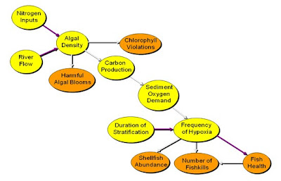
It is common modeling practice to develop a flow diagram consisting of “boxes and arrows” to describe relationships among key variables in an aquatic ecosystem and use this diagram as a device to guide model development and explanation. In ecology, this “graphical model” is typically used to display the flow of materials or energy in an ecosystem. For a probability network, however, the “flows” indicated by the arrows in a graphical model do not represent material flow or energy flow; rather, they represent conditional dependency. Thus, while the probability modeling approach of interest here typically begins with a graphical model, in this case the presence (absence) of an arrow connecting two boxes specifies conditional dependence (independence). An example is given in the figure below for eutrophication in the Neuse Estuary in North Carolina (Borsuk et al. 2004).

Probability networks like that in the figure can be as simple or as complex as scientific needs, knowledge, and data allow. The relationships may reflect direct causal dependencies based on process understanding or a statistical, aggregate summary of more complex associations. In either case, the relationships are characterized by conditional probability distributions that reflect the aggregate response of each variable to changes in its “up-arrow” (or parent) predecessor, together with the uncertainty in that response. In that regards, it is important to recognize that the conditional independence characterized by absence of an arrow in a Bayes net graphical model is not the same as complete independence, a feature that is likely to be quite rare in systems of interest. For example, ecological knowledge suggests that many of the variables in the figure are likely to be interrelated or interdependent. However, the arrows in the figure indicate that conditional on sediment oxygen demand and duration of stratification, frequency of hypoxia is independent of all other variables. This means that once sediment oxygen demand and duration of stratification are known, knowledge of other variables does not change the probability (frequency) of hypoxia.

Conditional probability relationships may be based on either (1) observational/experimental data or (2) expert scientific judgment. Observational data that consist of precise measurements of the variable or relationship of interest are likely to be the most useful, and least controversial, information. Unfortunately, appropriate and sufficient observational data may not always exist. Experimental evidence may fill this gap, but concerns may arise regarding the applicability of this information to the natural, uncontrolled system, and appropriate experimental data may also be limited. As a consequence, the elicited judgment of scientific experts may be required to quantify some of the probabilistic relationships (see: http://kreckhow.blogspot.com/2013/07/quantifying-expert-judgment-for.html). Of course, the use of subjective judgment is not unusual in water quality modeling. Even the most process-based computer simulations rely on subjective judgment as the basis for the mathematical formulations and the choice of parameter values. Therefore, the explicit use of scientific judgment in probability networks should be an acceptable practice. In fact, by formalizing the use of judgment through well-established techniques for expert assessment, the probability network method may improve the chances of accurate and honest predictions.

The Bayes net presented in the figure above as a graphical model was used for development of the TMDL (total maximum daily load) for nitrogen in the Neuse Estuary to address water quality standard violations (Borsuk et al. 2003). Several features of the Bayes net improved the modeling and analysis for the Neuse nitrogen TMDL. To facilitate explanations and to enhance credibility, the underlying structure of the Neuse probability network (reflected in the variables and relationships conveyed in the graphical model) is designed to be consistent with mechanistic understanding. The relationships in this model are probabilistic; they were estimated using a combination of optimization techniques and expert judgment. The predicted responses are also probabilistic, reflecting uncertainty in the model forecast. This is important, as it allows computation of a “margin of safety” which is required by the US EPA for the assessment of a total maximum daily load. In addition, the Bayes net model can be updated (using Bayes Theorem) as new information is obtained; this supports adaptive implementation, which is becoming an important strategy for successful environmental management.

Applications of Bayes nets are becoming more common in the environmental literature. Reckhow, Borsuk, and Stow (see Reckhow 1999, 2010, and Borsuk et al. 2003, 2004) present additional details documenting the Neuse Estuary Bayes net models described above, as well as Bayes nets developed and applied to address other issues. Software, both commercial and free, is available for development and application of Bayes nets; some examples are Hugin (http://www.hugin.com/), Netica (http://www.norsys.com/netica.html) BayesiaLab (http://www.bayesia.us/), and GeNIe (http://genie.sis.pitt.edu/).

Borsuk, Mark E., Craig A. Stow, and Kenneth H. Reckhow. 2003. An integrated approach to TMDL development for the Neuse River estuary using a Bayesian probability network model (Neu-BERN) . Journal Water Resources Planning and Management. 129:271-282.

https://www.researchgate.net/publication/238726404_Integrated_Approach_to_Total_Maximum_Daily_Load_Development_for_Neuse_River_Estuary_using_Bayesian_Probability_Network_Model_(Neu-BERN)?fulltextDialog=true&ev=prf_pub_xaddfulltext

Borsuk, M.E., C.A. Stow, and K.H. Reckhow. 2004. A Bayesian network of eutrophication models for synthesis, prediction, and uncertainty analysis. Ecological Modelling. 173:219-239.

https://www.researchgate.net/publication/228780081_Ecological_prediction_using_causal_Bayesian_networks_A_case_study_of_eutrophication_management_in_the_Neuse_River_estuary?ev=prf_pub

Reckhow, K.H. 1999. Water Quality Prediction and Probability Network Models. Canadian Journal of Fisheries and Aquatic Sciences.56:1150-1158.

https://www.researchgate.net/publication/2450055_Water_Quality_Prediction_and_Probability_Network_Models?ev=prf_pub

Reckhow, K.H. 2010. Bayesian Networks for the Assessment of the Effect of Urbanization on Stream Macroinvertebrates. Proceedings IEEE Computer Society Press. HICSS-43. Kauai, Hawaii.

https://www.researchgate.net/publication/221181371_Bayesian_Networks_for_the_Assessment_of_the_Effect_of_Urbanization_on_Stream_Macroinvertebrates?ev=prf_pub

Quantifying Expert Judgment for a Bayesian Analysis

In my view, one of the merits of a Bayesian analysis is the opportunity to develop a prior probability model using expert elicitation to express scientific knowledge. Expert elicitation involves a carefully-crafted interview process with a subject-area expert to translate an expert’s knowledge into a prior probability for a Bayesian analysis. For the elicitation, a specific strategy is recommended that involves: motivating, structuring, conditioning, encoding, and verifying:

·   Motivating (establishing rapport): This involves making sure that the expert has a comfortable understanding of the process.  This includes explaining the nature of problem and analysis, giving the expert context on how his or her judgments will be used, discussing the general methodology of a probabilistic assessment, explaining heuristics expert can use, and identifying any potential motivational biases.

·   Structuring (defining uncertain quantities): Once the expert is oriented as to the general what, how, and why, the next step is to clearly define the specific questions about which the expert will be providing judgment.  During this step, it is important to define variables of interest unambiguously and identify variable units as well as possible ranges of values. Variables can be disaggregated into more elementary variables, if necessary, or combined into summary variables, as appropriate.

·   Conditioning (thinking about all evidence): After the specific values to be elicited are chosen, the expert should then be prompted to think about all of his or her relevant expert knowledge concerning the variables and relationships of interest.  This knowledge could include data, theoretical models, analogies with similar systems, or other sources of understanding.  The expert should be encouraged to think from different perspectives and draw on as much information as possible in order to overcome potential biases related to consideration of limited scope.  For example, the elicitor can ask the expert to invent scenarios for extreme outcomes and ask the expert to explain how these different outcomes could occur.

·   Encoding  (quantifying expert judgment): After proper preparation in previous steps, this step comprises the actual elicitation.  Probabilistic information can be elicited according to many different proposed protocols, for example, the elicitor can fix the probability and directly elicit the variable value or conduct an indirect reference lottery.

·   Verifying (checking the answer): Finally, after all desired probabilities are encoded, the elicitor should test the expert answers given to see if they correctly capture the expert’s opinion.  This can be done by rephrasing an expert’s answer in another way to see if the expert still agrees with the assessment.  If the expert does not confirm the answer, the elicitor may need to repeat conditioning and encoding steps.

As an example, Reckhow (1988) used expert judgment to improve a model of fish population response to acid deposition in lakes when the knowledge of an expert is elicited and formally incorporated into the model using Bayes Theorem. In Reckhow’s study, an expert (Dr. Joan Baker) in fish response to acidification was interviewed to elicit a prior probability for the model parameters. The model was a logistic regression model with the form

where p(Presence) is the probability of species presence, b represents the model parameters, and x represents the predictor variables (pH and calcium).

Since with a statistical model, scientific experts are more likely to think in terms of the variables (pH, calcium, and species presence/absence) rather than in terms of the model parameters, a predictive distribution elicitation ap­proach was used to de­termine the prior probabilities. For this procedure, the expert was given a set of predictor variables and then asked to give her estimate of the median response. A frequency perspective was thought to facilitate response; thus a typical question was: “Given 100 lakes that have supported brook trout populations in the past, and if all 100 lakes have pH = 5.6 and calcium concentration = 130 ueq/L, what number do you now expect continue to support the brook trout population?” This question was repeat­ed 20 times with a variety of pH-calcium pairs to yield 20 predicted responses. Twenty was chosen to provide some re­dundancy to improve characterization of the prior yet not burden the expert with time-consuming questions. The pH-­calcium pairs were not randomly selected but rather were chosen to resemble the sample data matrix.

The expected response provided by Dr. Baker does not pro­vide a crucial measure of error. Thus, it was assumed that the errors in the conditional response were approximately nor­mally distributed, and additional questions were posed to Dr. Baker to determine fractiles of the predictive distribution, con­ditional on pH and calcium. A typical question was: “For pH = 5.1 and calcium = 90 ueq/L, you estimated that 55 lakes supported brook trout populations. If the odds are 3:1 that the number of lakes (of 100 total lakes) supporting brook trout is greater than a particular value, what is that value?” This question yields the 25th%, and other similar questions provide other percentiles. These fractiles were assessed for six conditional y [p(Presence)] distributions, producing six estimates for stan­dard error that are conditional on an assumed known un­derlying variance (estimated from the data). A thorough description of this probability elicitation and the complete Bayesian analysis can be found in Reckhow (1988).  

Kashuba, Roxolana, McMahon, Gerard, Cuffney, T.F., Qian, Song, Reckhow, Kenneth, Gerritsen, Jeroen, and Davies, Susan, 2012, Linking urbanization to the Biological Condition Gradient (BCG) for stream ecosystems in the Northeastern United States using a Bayesian network approach: U.S. Geological Survey Scientific Investigations Report 2012–5030, 48 p. (http://pubs.usgs.gov/sir/2012/5030/.)

Reckhow, K.H. 1988.  A Comparison of Robust Bayes and Classical Estimators for Regional Lake Models of Fish Response to Acidification. Water Resources Research. 24:1061-1068.

https://www.researchgate.net/publication/250310025_A_Comparison_of_Robust_Bayes_and_Classical_Estimaters_for_Regional_Lake_Models_of_Fish_Response_to_Acidification?ev=prf_pub

Bayesian Hypothesis Testing in Non-Replicated Studies

Many studies in ecology, both experimental and observational, are designed to assess what may be referred to as a “treatment effect.” The treatment effect can pertain to such things as: the influence of various factors on growth rate of an organism, the effect of a pollution control strategy on ambient pollutant concentrations, or the effect of a newly-created herbicide on animal life. It is common practice in these situations for the scientist to obtain data on the treatment effect and use hypothesis testing to assess the statistical significance of the effect.

In classical or frequentist statistical analysis, hypothesis testing for a treatment effect is often based on a point null hypothesis (which actually should be used only if it is considered appropriate from a scientific standpoint). Typically, the point null hypothesis is that there is no effect; it is often stated in this way as a “straw man” that the scientist expects to reject on the basis of the data evidence. To test the null hypothesis, data are obtained to provide a sample estimate of the effect of interest and then to compute an estimate of the test statistic. Following that, a table for the test statistic is consulted to assess how unusual the observed value of the test statistic is, given (assuming) that the null hypothesis is true. If the observed value of the test statistic is unusual, that is, if it essentially incompatible with the null hypothesis, then the null hypothesis is rejected.

In classical statistics, this assessment of the test statistic is based on the sampling distribution for the test statistic. The sampling distribution is a probability density function that is hypothetical is nature. In effect, it is a smoothed histogram for the test statistic plotted for a large number of hypothetical samples with the same sample size. Inference in classical statistics is based on the distribution of estimators and test statistics in many (hypothetical) samples, despite the fact that virtually all statistical investigations involve a single sample. This hypothetical sampling distribution provides a measure of the frequency, or probability, that a particular value, or range of values, for the test statistic will be determined for a set of many samples. In classical statistics, we equate this long-run frequency to the probability for a particular sample, before that sample is taken.

There are two problems with this approach that are addressed through use of Bayesian statistical methods. The first is that the hypothesis test is based on a test statistic that is at best indirectly related to the quantity of interest - the truth (or probability of truth) of the null hypothesis. The p-value commonly reported in hypothesis testing is the probability (frequency), given that the null hypothesis is true, of observing values for the test statistic that are as extreme, or more extreme, than the value actually observed; in other words:

p(test statistic equals or exceeds k|H₀ is true)                                    

The scientist, however, is interested in the probability of the correctness of the hypothesis, given that he has observed a particular value for the test statistic; in other words:

p(H₀ is true|test statistic=k)                                                                                    

Classical statistical inference does not provide a direct answer to the scientist's question; Bayesian inference does.

The second problem relates to the issue of “conditioning,” which concerns the nature of the sample information in support of the hypothesis. Bayesian hypothesis tests are conditioned only on the sample taken, whereas classical hypothesis tests are conditioned on other hypothetical samples in the sampling distribution (more extreme than that observed) that could have been selected, but were not. The Bayesian approach, of course, uses more than the sample as it also incorporates prior information. However, the prior, while judgmental, does relate to the hypothesis of interest, whereas the sampling distribution relates to logically irrelevant, hypothetical samples. Clearly, the Bayesian approach is more focused on the problem of interest to the ecologist.

Reckhow (1990) illustrates the tendency of p-values to overstate the sample evidence against the null hypothesis in an example concerning acidification of lakes.

 Reckhow, K.H. 1990.  Bayesian Inference in Non-Replicated Ecological Studies.  Ecology. 71:2053-2059.

https://www.researchgate.net/publication/249011176_Bayesian_Inference_in_Non-Replicated_Ecological_Studies?ev=prf_pub

Should TMDL Modeling Include Uncertainty Analysis?

Will TMDL decisions  be improved with knowledge of the uncertainty in outcomes from proposed pollutant load reductions? That is, will our decisions generally be better if we have some idea of the range of possible outcomes that might result? I believe that the answer is yes, and yet current practice in water quality assessment and management suggests that others may believe that decision making might be undermined with full disclosure of uncertainties, or perhaps believe that uncertainty is small enough that it can be safely ignored.

Despite these reservations, it is noteworthy that the U.S. EPA also believes the answer is ‘‘yes,’’ although their reasoning is unclear. EPA’s perspective is implicit in their technical requirement for an uncertainty-based ‘‘margin of safety’’ (MOS) in a TMDL application; however, absent from EPA guidance is an explanation as to why decisions improve with an uncertainty analysis.

Despite the requirement for an uncertainty-based MOS estimate, few TMDLs are accompanied by actual estimates of forecast uncertainty. Instead, TMDLs are typically proposed with either ‘‘conservative’’ modeling assumptions or an arbitrarily chosen MOS (often implemented as an additional 10% pollutant load reduction). Neither approach explicitly links the MOS to TMDL forecast uncertainty. However, by hedging the TMDL decision in the direction of environmental protection, the MOS effectively increases the assurance that water quality standards will be achieved. This may seem reasonable and even desirable, but it must be noted that this hedging comes at a cost, and the basis for the hedging cost is totally arbitrary in most cases.

The National Research Council Committee to Assess the Scientific Basis of the Total Maximum Daily Load Approach to Water Pollution Reduction has recognized the arbitrary way in which the margin of safety has been applied. Specifically, their Executive Summary contains the following recommendation (National Research Council (NRC). (2001). Assessing the TMDL approach to water quality management, National Academy Press, Washington, D.C.):

The TMDL program currently accounts for the uncertainty embedded in the modeling exercise by applying a Margin of Safety (MOS); EPA should end the practice of arbitrary selection of the MOS and instead require uncertainty analysis as the basis for MOS determination.

However, acknowledging and computing model prediction uncertainty is not without challenges, as I learned many years ago. While in graduate school, I became involved in a proposed consulting venture in New Hampshire focusing on 208 planning. As a young scientist, I was eager to apply my new scientific knowledge, so I suggested to my consulting colleagues that we add uncertainty analysis to our proposed 208 study; everyone agreed. After we made our presentation to the client, perhaps predictably the client’s first question was, ‘‘the previous consultants didn’t mention uncertainty in their proposed modeling study, what’s wrong with your model?’’ This experience made me realize that I had much to learn about the role of science in decision making and about effective presentations!

While this story may give the impression that I’m being critical of the client for not recognizing the ubiquitous uncertainty in environmental forecasts, in fact I believe the fault to lie primarily with the scientists and engineers who fail to fully inform clients of the uncertainty in their assessments. Partially in their defense, water quality modelers may not see why decision makers are better off knowing the forecast uncertainty, and perhaps modelers may not want to be forced to answer the embarrassing question like the one posed to me years ago in New Hampshire.

For this situation to change, that is, for decision makers to demand estimates of forecast error, decision makers first need (1) motivation—that is, they must become aware of the substantial magnitude of forecast error in many water quality assessments, and (2) guidance—ideally, they need relatively simple heuristics that will allow them to use this knowledge of forecast error to improve decision making in the long run. Once this happens, and decision makers demand that water quality forecasts be accompanied with error estimates, water quality modelers can support this need through distinct short-term and long-term strategies.

Short-term approaches are necessary since existing mechanistic water quality models are over-parameterized and thus not supportive of a complete error analysis. Thus procedures are needed to immediately (1) conduct an informative, but incomplete error analysis, and (2) use that incomplete error analysis to improve decision making. In the long term, recommendations can be made to (1) restructure the models so that a relatively complete error analysis is feasible, and (2) employ Bayesian approaches that are compatible with adaptive assessment techniques that provide the best approach for improving forecasts over time.

In the short term, if knowledge, data, or model structure prevents uncertainty analysis from being complete, is there any value in conducting an incomplete uncertainty analysis? Stated another way, is it reasonable that decision making will be improved with even partial information on uncertainties, in comparison to current practice with no reporting of prediction uncertainties? Often, but not always, the answer is ‘‘yes,’’ although the usefulness of incomplete uncertainty characterization, like the analysis itself, is limited.

Using decision analysis as a prescriptive model, we know that uncertainty analysis can improve decision making when prediction uncertainty is integrated with the utility (or loss, damage, net benefits) function to allow decision makers to maximize expected utility (or maximize net benefits). When uncertainty analysis is incomplete (and perhaps more likely, the utility function is poorly characterized) the concepts of decision analysis may still provide a useful guide.

For example, triangular distributions could be assessed for all uncertain model terms, and then ignoring correlation between model parameters, limited systematic sampling (e.g., Latin hypercube) from these distributions could be used to simulate the prediction error. The result of this computation could be either over- or underestimation of error, but it would provide some indication of error magnitude. However, this information alone, while perhaps helpful for research and monitoring needs, does not aid decision making. The approximate estimates of prediction uncertainty need to be considered in conjunction with the attitudes toward risk for the key decision variables.

Implicit in this attitude toward risk is an expression of preferences regarding trade-offs. For example, are decision makers sufficiently risk-averse concerning noncompliance with a water quality standard and its associated designated use, such that they are willing to increase pollutant control costs in order to increase the chance of attainment of certain water uses? Suppose a reasonable quantification of prediction uncertainty were available for a fecal coliform water quality criterion and its designated use of commercial shellfishing. Then alternative TMDL predictions might be expressed as ‘‘there’s a 40% chance of loss of commercial shell- fishing with plan A, but only a 5% chance of loss with plan B.’’ When costs of the plans are considered in conjunction with these uncertain TMDL forecasts, the trade-off between shellfishing loss and cost may be enhanced by awareness of risk that comes from the prediction uncertainty estimates. Since risk is not evident from deterministic (point) predictions of the decision attributes, the decision is likely to be better informed with risk assessment made possible through estimation of prediction uncertainty.

Given the components of a TMDL, how might the requirement for uncertainty analysis change the TMDL analysis and selection process? The TMDL margin of safety is protective in one direction only: it is protective of the environment, but at the possible unnecessary expense of pollution control overdesign. Thus, knowledge of prediction uncertainty and risk attitudes can be helpful primarily in determining the magnitude (not direction) of the margin of safety. One strategy, therefore, is to set the MOS as a multiplier of the TMDL prediction uncertainty, with the magnitude of this multiplier reflecting the risk assessment discussed above.

In the long run, the best strategy for TMDL forecasting and assessment will probably be to restructure the models, emphasizing the development of techniques that are compatible with the need for error propagation and adaptive implementation. Adaptive TMDLs, following an adaptive management format, make use of post-implementation monitoring data to assess standards compliance. Under adaptive implementation, if the data imply that water quality standards will not be met, then adjustments can be made to the TMDL implementation plan.

Of course, this raises another issue concerning uncertainty that warrants comment. Specifically, even the best compliance monitoring involves sampling a population, which implies sampling error. That does not even begin to cover standards compliance assessment based on no water quality data (just expert judgment alone) or methods to assess compliance with narrative standards. All of these imply uncertainties in the 303(d) listing of impaired waters in need of a TMDL. For compliance assessment, the solution seems clear. States should translate any narrative water quality standards into quantitative metrics, and they should employ statistical hypothesis testing with water quality data to rigorously assess compliance.

While acknowledging the error in monitoring data, I nonetheless believe that the use of adaptive implementation is a prudent response to the large forecast errors expected using current water quality models. In brief, if TMDL forecasts may be substantially in error, then corrections for these TMDLs are likely to be necessary. In that situation, recognition and accommodation at the initiation of the TMDL, allowing for refinement of the TMDL over time, is a pragmatic strategy. Since analytic approaches supporting adaptive implementation are likely to be based on combining initial TMDL forecasts with post-implementation monitoring, error terms are needed for both the model forecasts and the monitoring data to efficiently combine forecasts with observations in order to adaptively update the TMDL forecast. Bayesian (probability) networks are particularly suitable for this task.

In conclusion, estimation of TMDL forecast uncertainty should not be a requirement merely because the margin of safety requires it. Rather, uncertainty should be computed because it results in better decisions. In the short run, this can happen when the TMDL assessment is based on considerations of risk. In the long run, adaptive implementation should improve the TMDL program, and effective use of adaptive implementation is facilitated with uncertainty analysis. Regardless of time frame, the TMDL program will be better served with complete estimates of uncertainty than with arbitrary hedging factors that simply fulfill an administrative requirement.